環境
Windows10(1903)のWSL(Ubuntu 18.04)とJupyter Notebookを使用。
Pyhtonライブラリのインストール
pyLDAvisとUMAP用のライブラリUMAP-learnをインストールする。
インストールされたバージョンは以下の通り。
pyLDAvisのソースコードの改修
まずはPythonライブラリなどがインストールされているディレクトリを確認する。ホームディレクトリ内の「.local/lib/python3.6/site-packages」がそのディレクトリで、その配下にpyLDAvisというディレクトリがある。修正するのはpyLDAvisディレクトリ内の_prepare.py。
pyLDAvisではscikit-learn(sklearn.manifold.TSNE)でt-SNEによる次元削減を行っている。UMAP-learnはTSNEクラスと同様の書式で使えるので、基本的にはTSNE用のコードを参考にUMAP用のコードを追加する。
TSNEではパラメータのmetricで距離の計算方法を指定でき、それはUMAP-learnでも同じ。ただし、pyLDAvisでは独自の関数で定義したJensen-Shannonダイバージェンスを距離の計算に使用しており、TSNEのパラメータmetricに「precomputed」を指定して計算済みのデータを渡している。UMAP-learnのドキュメントにはmetricに「precomputed」はないが、Does UMAP accept a distance matrix as custom metric?によると、バージョン0.2以降では対応しているらしい。
上記をふまえて、_prepare.pyを以下のように変更する。
# 23行目に以下を追記
try:
    from umap import UMAP
    umaplearn_present = True
except ImportError:
    umaplearn_present = False

# js_TSNE関数の後(170行目あたり)に以下を追記
def js_UMAP(distributions, **kwargs):
    """Dimension reduction via UMAP

    Parameters
    ----------
    distributions : array-like, shape (`n_dists`, `k`)
        Matrix of distributions probabilities.

    **kwargs : Keyword argument to be passed to `umap.UMAP()`

    Returns
    -------
    umap : array, shape (`n_dists`, 2)
    """

    dist_matrix = squareform(pdist(distributions, metric=_jensen_shannon))
    model = UMAP(n_components=2, metric='precomputed', random_state=0, **kwargs)
    return model.fit_transform(dist_matrix)

# 382行(mds = js_PCoAの次の行)に以下を追記
        elif mds == 'umap':
            if umaplearn_present:
                mds = js_UMAP
            else:
                logging.warning('umap-learn not present, switch to PCoA')
                mds = js_PCoA
データセットの準備
改修したpyLDAvisを試すために、株式会社 ロンウイットが公開しているlivedoor ニュースコーパス(通常テキスト:ldcc-20140209.tar.gz )を使用してgensimでLDAモデルを作成する。ダウンロードして解凍するとtextディレクトリ配下にニュースカテゴリーごとに9のディレクトリがある。それぞれのディレクトリ内には記事ごとのテキストファイルがある。
記事ごとのテキストファイルについては、textディレクトリ配下のREADME.txtにフォーマットの説明がある。
1行目:記事のURL
2行目:記事の日付
3行目:記事のタイトル
4行目以降:記事の本文
以下のPyhtonスクリプトで、記事テキストを読み込んでPandasのデータフレームにしてpickle形式で保存する。
import os
import glob
import re
import csv
from datetime import datetime

import pandas as pd

# ニュースカテゴリーのディレクトリ名
NEWS_CATEGORY = ['it-life-hack', 'movie-enter', 'sports-watch', 'kaden-channel', 'peachy', 'topic-news', 'dokujo-tsushin', 'livedoor-homme', 'smax']

def clean(text):
    # テキストのクリーニング

    text = text.strip()

    # ■関連リンク/サイト/ニュース/記事/情報 以降の削除
    res = re.split('■関連', text)

    if len(res) > 1:
        text = res[0]

    # 【関連情報】/【関連記事】 以降の削除
    res = re.split('【関連情報】|【関連記事】', text)
    if len(res) > 1:
        text = res[0]

    # メールアドレス削除
    text = re.sub('[a-zA-Z0-9.!#$%&\'*+\/=?^_`{|}~-]+@[a-zA-Z0-9-]+(?:\.[a-zA-Z0-9-]+)*', '', text)

    # URL削除
    text = re.sub('https?://[\w!?/\+\-_~=;\.,*&@#$%\(\)\'\[\]]+', '', text)

    # ~年~月~日を削除
    text = re.sub('[0-9]{1,2}月|[0-9]{1,2}日|[0-9]{2,4}年', '', text)

    return text

def main():
    df = pd.DataFrame()
    for category in NEWS_CATEGORY:
        path = os.path.join('text', category, '{}-*.txt'.format(category))

        txtpaths = glob.glob(path)

        for txtfile in txtpaths:
            with open(txtfile, mode='r') as f:
                # URL
                url= f.readline().strip()

                # 日付
                dt = datetime.strptime(f.readline().split('+')[0].strip(), "%Y-%m-%dT%H:%M:%S")

                # 記事タイトル
                title= f.readline().strip()

                # 記事テキスト
                txt = f.read().strip()

            df = df.append([[category, url, dt, title, clean(txt)]], ignore_index=True)

    columns = ['category', 'url', 'date', 'title', 'body']
    df.columns = columns

    print(df.info())
    print(df.head())
    df.to_pickle('news.pkl')

if __name__ == '__main__':
    main()
上記スクリプトを実行して作成されたデータフレームには7367件のデータがある。
LDAモデルの作成
作成したデータフレーム内のテキストをMeCabで形態素解析して、gensimでLDAモデルを作成するスクリプトを用意する。今回は名詞、動詞、形容詞、副詞のみを使用し、LDAのトピック数はニュースカテゴリー数の9とする。
import pandas as pd

import MeCab
from gensim.corpora import Dictionary
from gensim.models import LdaModel

POS_LIST = ['名詞', '動詞', '形容詞', '副詞']
STOP_LIST = ['*']

m = MeCab.Tagger('-Ochasen')
m.parse('')

def text2list(text):
    # 形態素の原形リストを取得する

    node = m.parseToNode(text)
    term_l = []
    while node:
        feature_split = node.feature.split(',')

        pos1 = feature_split[0]
        base_form = feature_split[6]

        if pos1 in POS_LIST and base_form not in STOP_LIST:
            term_l.append(base_form)

        node = node.next

    return term_l

def ldamodel(text_2l, n_topics):
    # LDAモデルの作成

    dct =  Dictionary(text_2l)

    # no_below: no_belowを下回るドキュメント数にしか含まれない語を除外
    # no_above: 語を含む文書数/全文書数 がno_aboveを上回る語を除外
    dct.filter_extremes(no_below=5, no_above=0.7)

    # コーパスの作成
    corpus = [dct.doc2bow(text) for text in text_2l]

    # ニュースカテゴリー数をトピック数に指定してモデル作成
    model = LdaModel(corpus=corpus, num_topics=n_topics, minimum_probability=0.0, id2word=dct, random_state=1,
        alpha='auto', eta='auto', chunksize=1500, passes=2)

    return model, corpus, dct

def build_model():
    # 保存しておいたニュースのDataFrameの読み込み
    df = pd.read_pickle('news.pkl')

    # ニュースカテゴリー数
    n_categories = df['category'].nunique()

    # ニュース記事テキストを形態素解析してリストにする
    df['term_l'] = df['body'].apply(text2list)

    # LDAモデル作成
    return ldamodel(df['term_l'].tolist(), n_categories)
上記のLDAモデルを作成するスクリプト(lda_news.py)とニュース記事のデータフレーム(news.pkl)を同じディレクトリ(news)に置いておく。
pyLDAvisとUMAPでLDAを可視化する
準備が整ったので、修正したpyLDAvisでLDAの結果をJupyter Notebookで可視化してみようと思ったが、Jupyter Notebook上で表示できなかったのでhtmlに出力する(pyLDAvisを修正していない状態でも同じなので、今回の修正の影響ではない)。
import pyLDAvis
import pyLDAvis.gensim
pyLDAvis.enable_notebook()

# 実行ディレクトリをlda_news.pyとnews.pklがあるディレクトリに変更
import os
from pathlib import Path
home = str(Path.home())
os.chdir(os.path.join(home, 'news'))

from lda_news import build_model

model, corpus, dct = build_model()

# mdsに追加した「umap」を指定
vis = pyLDAvis.gensim.prepare(model, corpus, dct, mds='umap', sort_topics=False)

# htmlに出力
pyLDAvis.save_html(vis, 'lda.html')
UMAPで可視化した結果は以下の通り。
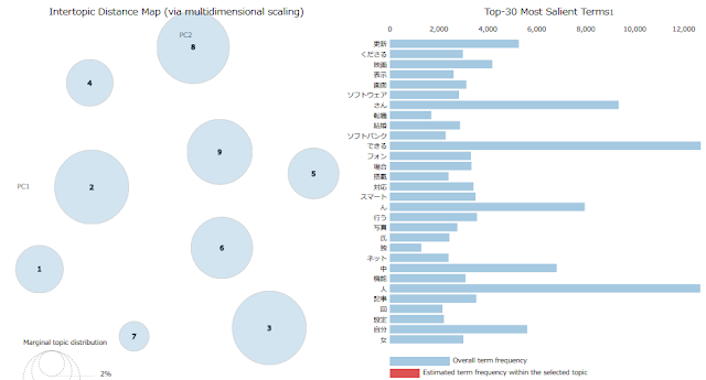
続いてt-SNEでの可視化の結果。
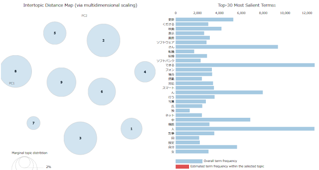
UMAPのほうがt-SNEよりも実行時間が短くなるのではと期待していたが、実際にはほとんど同じだった。もっと大規模なデータセットでないと差がでないのだろうか。
0 件のコメント:
コメントを投稿